Heisenberg picture
| Quantum mechanics |
|---|
 |
| Introduction Glossary · History |
|
Background
|
|
Fundamental concepts
|
|
Formulations
|
|
Equations
|
|
Advanced topics
|
|
Scientists
Bell · Bohm · Bohr · Born · Bose
de Broglie · Dirac · Ehrenfest Everett · Feynman · Heisenberg Jordan · Kramers · von Neumann Pauli · Planck · Schrödinger Sommerfeld · Wien · Wigner |
In physics, the Heisenberg picture is a formulation of quantum mechanics in which the operators (observables and others) incorporate a dependency on time, but the state vectors are time-independent. It stands in contrast to the Schrödinger picture in which the operators are constant and the states evolve in time. The two models only differ by a basis change with respect to time-dependency, which is the difference between active and passive transformation. The Heisenberg picture is the formulation of matrix mechanics in an arbitrary basis, in which the Hamiltonian is not necessarily diagonal.
Contents |
Mathematical details
In the Heisenberg picture of quantum mechanics the state vector,  , does not change with time, and an observable A satisfies
![\frac{d}{dt}A(t)={i \over \hbar}[H,A(t)]%2B\left(\frac{\partial A}{\partial t}\right)(t),](/2012-wikipedia_en_all_nopic_01_2012/I/4eb187665838af8fbac6a05942df54f8.png)
where H is the Hamiltonian and [·,·] is the commutator of A and H. In some sense, the Heisenberg picture is more natural and fundamental than the Schrödinger picture, especially for relativistic theories. Lorentz invariance is manifest in the Heisenberg picture.
This approach has a similarity to classical physics: by replacing the commutator above by the Poisson bracket, the Heisenberg equation becomes an equation in Hamiltonian mechanics.
By the Stone-von Neumann theorem, the Heisenberg picture and the Schrödinger picture are unitarily equivalent.
Deriving Heisenberg's equation
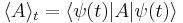
The expectation value of an observable A, which is a Hermitian linear operator, for a given state  is given by:
In general 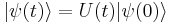 where
where 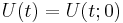 is the time evolution operator. For an elementary derivation, we will take Hamiltonian to commute with itself at different times, and further, be independent of time, in which case it simplifies to
where H is the Hamiltonian and ħ is Planck's constant divided by  . It follows that

With the definition,
it follows:

(differentiating according to the product rule) noting that  is the time derivative of A(t), the transformed operator, not the one we started with.

The last passage is valid since : commutes with H. From this results the Heisenberg equation of motion:
![{d \over dt} A(t) = {i \over \hbar } [ H , A(t) ] %2B \left(\frac{\partial A}{\partial t}\right)(t)](/2012-wikipedia_en_all_nopic_01_2012/I/aa28c6ddd20bc79bc06629cf19e603ac.png) ,
,
where [X, Y] is the commutator of two operators and defined as [X, Y] := XY − YX.
Now, using the operator identity
![{e^B A e^{-B}} = A %2B [B,A] %2B \frac{1}{2!} [B,[B,A]] %2B \frac{1}{3!}[B,[B,[B,A]]]%2B\cdots](/2012-wikipedia_en_all_nopic_01_2012/I/52e98fb39560666850c75a3ed12b9679.png)
one obtains for an observable A:
![A(t)=A%2B\frac{it}{\hbar}[H,A]-\frac{t^{2}}{2!\hbar^{2}}[H,[H,A]]
- \frac{it^3}{3!\hbar^3}[H,[H,[H,A]]] %2B \dots.](/2012-wikipedia_en_all_nopic_01_2012/I/5ad90caa8dd9acd7703e840d74d45a7e.png)
Due to the relationship between Poisson Bracket and Commutators this relation also holds for classical mechanics.
note: the relationship between Poisson Bracket and Commutators is
![[A,H]=i\hbar\{A,H\}](/2012-wikipedia_en_all_nopic_01_2012/I/15eb45c59d8552ca9aff71e7aee095ad.png)
in classical mechanics
so you can convince yourself that A(t) equation is the Taylor expansion on t=0
Commutator relations
Obviously, commutator relations are quite different than in the Schrödinger picture because of the time dependency of operators. For example, consider the operators  and
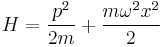
and  . The time evolution of those operators depends on the Hamiltonian of the system. For the one-dimensional harmonic oscillator
The evolution of the position and momentum operators is given by:
![{d \over dt} x(t) = {i \over \hbar } [ H , x(t) ]=\frac {p}{m}](/2012-wikipedia_en_all_nopic_01_2012/I/e88241a3ed0c7b4d98dead7c4db7fb7b.png)
![{d \over dt} p(t) = {i \over \hbar } [ H , p(t) ]= -m \omega^{2} x](/2012-wikipedia_en_all_nopic_01_2012/I/8e34c9dec77f73711b621179615fca2e.png)
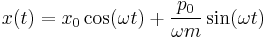
By differentiating both equations one more time and solving them with proper initial conditions
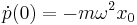

leads to:

Now, we are ready to directly compute the commutator relations:
![[x(t_{1}), x(t_{2})]=\frac{i\hbar}{m\omega}\sin(\omega t_{2}-\omega t_{1})](/2012-wikipedia_en_all_nopic_01_2012/I/4ae22c502c3f0a17595d025e1ea09259.png)
![[p(t_{1}), p(t_{2})]=i\hbar m\omega\sin(\omega t_{2}-\omega t_{1})](/2012-wikipedia_en_all_nopic_01_2012/I/93d155bb1d30982de6faa067f12f3c97.png)
![[x(t_{1}), p(t_{2})]=i\hbar \cos(\omega t_{2}-\omega t_{1})](/2012-wikipedia_en_all_nopic_01_2012/I/6d9e9d40904eacf630d54959ef5cb9b4.png)
For  , one simply gets the well-known canonical commutation relations.
See also
Further reading
- Cohen-Tannoudji, Claude; Bernard Diu, Frank Laloe (1977). Quantum Mechanics (Volume One). Paris: Wiley. pp. 312–314. ISBN 047116433X.
External links
- Pedagogic Aides to Quantum Field Theory Click on the link for Chap. 2 to find an extensive, simplified introduction to the Heisenberg picture.